44 how to display data labels in excel
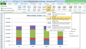
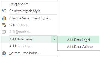
How to add data labels from different column in an Excel chart? This method will introduce a solution to add all data labels from a different column in an Excel chart at the same time. Please do as follows: 1. Right click the data series in the chart, and select Add Data Labels > Add Data Labels from the context menu to add data labels. 2. Display Missing Dates in Excel PivotTables - My Online Training … Mar 25, 2014 · A regular PivotTable will only display the dates present in the source data. If you want to display the missing dates for March you need to take the following convoluted steps: Right-click one of the date row labels in the PivotTable > select Group > Days and Months:
› documents › excelHow to display text labels in the X-axis of scatter chart in ... Select the data you use, and click Insert > Insert Line & Area Chart > Line with Markers to select a line chart. See screenshot: 2. Then right click on the line in the chart to select Format Data Series from the context menu. See screenshot: 3. In the Format Data Series pane, under Fill & Line tab, click Line to display the Line section, then ...
How to display data labels in excel
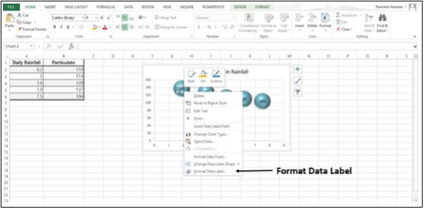
Edit titles or data labels in a chart - support.microsoft.com To reposition all data labels for an entire data series, click a data label once to select the data series. To reposition a specific data label, click that data label twice to select it. This displays the Chart Tools , adding the Design , Layout , and Format tabs. Format Data Labels in Excel- Instructions - TeachUcomp, Inc. Nov 14, 2019 · Then select the “Format Data Labels…” command from the pop-up menu that appears to format data labels in Excel. Using either method then displays the “Format Data Labels” task pane at the right side of the screen. Format Data Labels in Excel- Instructions: A picture of the “Format Data Labels” task pane in Excel. Excel tutorial: How to use data labels Generally, the easiest way to show data labels to use the chart elements menu. When you check the box, you'll see data labels appear in the chart. If you have more than one data series, you can select a series first, then turn on data labels for that series only. You can even select a single bar, and show just one data label.
How to display data labels in excel. › charts › dynamic-chart-dataCreate Dynamic Chart Data Labels with Slicers - Excel Campus Feb 10, 2016 · Typically a chart will display data labels based on the underlying source data for the chart. In Excel 2013 a new feature called “Value from Cells” was introduced. This feature allows us to specify the a range that we want to use for the labels. Since our data labels will change between a currency ($) and percentage (%) formats, we need a ... How to display text labels in the X-axis of scatter chart in Excel? Select the data you use, and click Insert > Insert Line & Area Chart > Line with Markers to select a line chart. See screenshot: 2. Then right click on the line in the chart to select Format Data Series from the context menu. See screenshot: 3. In the Format Data Series pane, under Fill & Line tab, click Line to display the Line section, then ... › documents › excelHow to add data labels from different column in an Excel chart? Click any data label to select all data labels, and then click the specified data label to select it only in the chart. 3. Go to the formula bar, type =, select the corresponding cell in the different column, and press the Enter key. See screenshot: 4. Repeat the above 2 - 3 steps to add data labels from the different column for other data points. How to Use Cell Values for Excel Chart Labels Select the chart, choose the "Chart Elements" option, click the "Data Labels" arrow, and then "More Options." Uncheck the "Value" box and check the "Value From Cells" box. Select cells C2:C6 to use for the data label range and then click the "OK" button. The values from these cells are now used for the chart data labels.
Excel, giving data labels to only the top/bottom X% values Here is what you can do, in stages: 1) Create a data set next to your original series column with only the values you want labels for (again, this can be formula driven to only select the top / bottom n values). See column D below. 2) Add this data series to the chart and show the data labels. How To Display Data Labels In Excel Chart - gfecc.org Adding Rich Data Labels To Charts In Excel 2013 Microsoft; Improve Your X Y Scatter Chart With Custom Data Labels; Data Label Sada Margarethaydon Com; Enable Or Disable Excel Data Labels At The Click Of A Button; How To Add Label Leader Lines To An Excel Pie Chart Excel; Adding Rich Data Labels To Charts In Excel 2013 Microsoft; Show Trend ... Change the format of data labels in a chart To get there, after adding your data labels, select the data label to format, and then click Chart Elements > Data Labels > More Options. To go to the appropriate area, click one of the four icons ( Fill & Line, Effects, Size & Properties ( Layout & Properties in Outlook or Word), or Label Options) shown here. How to Print Labels From Excel - Lifewire Choose Start Mail Merge > Labels . Choose the brand in the Label Vendors box and then choose the product number, which is listed on the label package. You can also select New Label if you want to enter custom label dimensions. Click OK when you are ready to proceed. Connect the Worksheet to the Labels
How to show data label in "percentage" instead of - Microsoft Community Select Format Data Labels Select Number in the left column Select Percentage in the popup options In the Format code field set the number of decimal places required and click Add. (Or if the table data in in percentage format then you can select Link to source.) Click OK Regards, OssieMac Report abuse 8 people found this reply helpful · Custom Chart Data Labels In Excel With Formulas Follow the steps below to create the custom data labels. Select the chart label you want to change. In the formula-bar hit = (equals), select the cell reference containing your chart label's data. In this case, the first label is in cell E2. Finally, repeat for all your chart laebls. Excel charts: add title, customize chart axis, legend and data labels ... For this, click the arrow next to Data Labels, and choose the option you want. To show data labels inside text bubbles, click Data Callout. How to change data displayed on labels To change what is displayed on the data labels in your chart, click the Chart Elements button > Data Labels > More options… How To Create Labels In Excel - Wachagghana News Then Click The Chart Elements, And Check Data Labels, Then You Can Click The Arrow To Choose An Option About The Data Labels In The Sub Menu.see Screenshot: Arrange the layout of your address labels. Type equals (=) and then the up arrow to enter a formula with a direct cell reference to the first data label.
How to Add Data Labels in Excel - Excelchat | Excelchat
Make Chart X Axis Labels Display below Negative Data - Excel … Aug 21, 2018 · #2 right click on the selected X Axis, and select Format Axis…from the pop-up menu list. The Format Axis pane will be displayed in the right of excel window. #3 on Format Axis pane, expand the Labels section, select Low option from the Label Position drop-down list box. Close the Format Axis pane.

32 Data Label Excel - Labels Design Ideas 2020
Excel charts: how to move data labels to legend - Microsoft Tech Community @Matt_Fischer-Daly . You can't do that, but you can show a data table below the chart instead of data labels: Click anywhere on the chart. On the Design tab of the ribbon (under Chart Tools), in the Chart Layouts group, click Add Chart Element > Data Table > With Legend Keys (or No Legend Keys if you prefer)
How to Show Percentages in Stacked Bar and Column Charts in Excel
How to Add Data Labels to an Excel 2010 Chart - dummies On the Chart Tools Layout tab, click Data Labels→More Data Label Options. The Format Data Labels dialog box appears. You can use the options on the Label Options, Number, Fill, Border Color, Border Styles, Shadow, Glow and Soft Edges, 3-D Format, and Alignment tabs to customize the appearance and position of the data labels.

How to create Custom Data Labels in Excel Charts - Efficiency 365
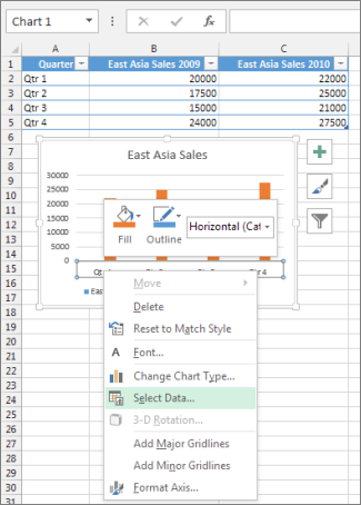
Add or remove data labels in a chart - support.microsoft.com Right-click the data series or data label to display more data for, and then click Format Data Labels. Click Label Options and under Label Contains , select the Values From Cells checkbox. When the Data Label Range dialog box appears, go back to the spreadsheet and select the range for which you want the cell values to display as data labels.

Creating Pie Chart and Adding/Formatting Data Labels (Excel) - YouTube
How to use data labels in a chart - YouTube Excel charts have a flexible system to display values called "data labels". Data labels are a classic example a "simple" Excel feature with a huge range of o...

Show Trend Arrows in Excel Chart Data Labels
chandoo.org › wp › change-data-labels-in-chartsHow to Change Excel Chart Data Labels to Custom Values? May 05, 2010 · Now, click on any data label. This will select “all” data labels. Now click once again. At this point excel will select only one data label. Go to Formula bar, press = and point to the cell where the data label for that chart data point is defined. Repeat the process for all other data labels, one after another. See the screencast.

Microsoft Excel Tutorials: The Chart Layout Panels
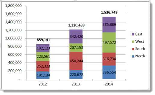
How to Add Data Labels in Excel - Excelchat | Excelchat After inserting a chart in Excel 2010 and earlier versions we need to do the followings to add data labels to the chart; Click inside the chart area to display the Chart Tools. Figure 2. Chart Tools Click on Layout tab of the Chart Tools. In Labels group, click on Data Labels and select the position to add labels to the chart. Figure 3.

Enable or Disable Excel Data Labels at the click of a button - How To - PakAccountants.com
Adding Data Labels to Your Chart (Microsoft Excel) Make sure the Design tab of the ribbon is displayed. (This will appear when the chart is selected.) Click the Add Chart Element drop-down list. Select the Data Labels tool. Excel displays a number of options that control where your data labels are positioned. Select the position that best fits where you want your labels to appear.
Charts in Excel - Easy Excel Tutorial
Excel 2010: Show Data Labels In Chart - AddictiveTips Lets look at how to enable and use them. To enable data labels in chart, select the chart and head over to Chart Tools Layout tab, from Labels group, under Data Labels options, select a position. It will show Data labels at specified position. Likewise, from Data Labels pull-down menu, you can change the position of data labels and access other ...

Automatically update data labels on Excel chart (Excel 2016) - Stack Overflow
peltiertech.com › select-data-display-in-excelSelect Data to Display in an Excel Chart With Option Buttons Feb 17, 2015 · My suggested approach will add some columns (F:I) to the existing data range with formulas that show or don’t show data based on which of two option buttons is selected, and my chart will use all of this data. When the formulas don’t show the values, they will not appear in the chart. The Data. The extended data range is shown below.
ExcelQuickPages
Chart: Display alternative values as Data Labels or Data Callouts - MrExcel Joined. Aug 11, 2017. Messages. 1. Aug 11, 2017. #1. Below is my excel chart. I would like to add a "data labels" or "data callouts". As you can see the line is displaying the data from Actual X and Y, but I want to display the DEV values on this line.
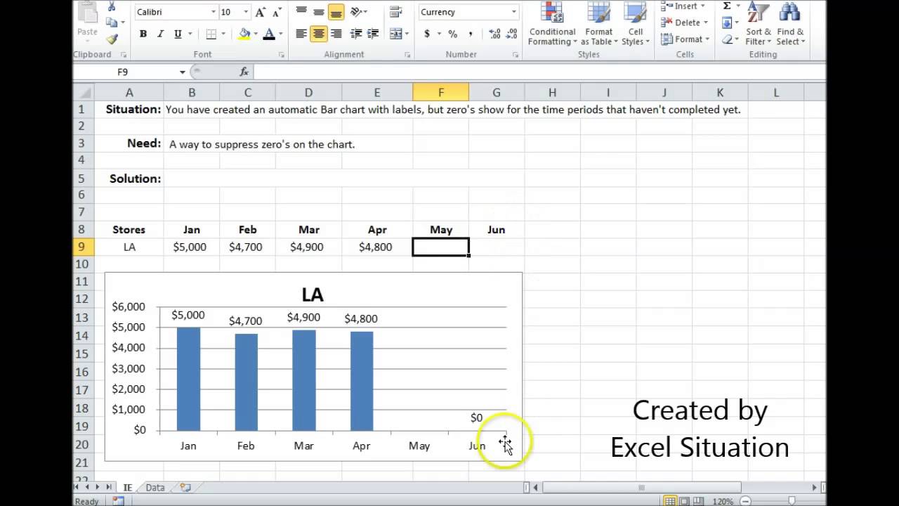
Excel Bar Chart Suppress Zeros - YouTube
Create Dynamic Chart Data Labels with Slicers - Excel Campus Feb 10, 2016 · Typically a chart will display data labels based on the underlying source data for the chart. In Excel 2013 a new feature called “Value from Cells” was introduced. This feature allows us to specify the a range that we want to use for the labels. Since our data labels will change between a currency ($) and percentage (%) formats, we need a ...

Chart Data Labels in PowerPoint 2011 for Mac
How to find, highlight and label a data point in Excel scatter plot Select the Data Labels box and choose where to position the label. By default, Excel shows one numeric value for the label, y value in our case. To display both x and y values, right-click the label, click Format Data Labels…, select the X Value and Y value boxes, and set the Separator of your choosing: Label the data point by name

Callout Data Labels for Charts in PowerPoint 2013 for Windows
Select Data to Display in an Excel Chart With Option Buttons Feb 17, 2015 · My suggested approach will add some columns (F:I) to the existing data range with formulas that show or don’t show data based on which of two option buttons is selected, and my chart will use all of this data. When the formulas don’t show the values, they will not appear in the chart. The Data. The extended data range is shown below.
Creating a chart with dynamic labels - Microsoft Excel 2013
Quick Tip: Excel 2013 offers flexible data labels | TechRepublic right-click and choose Insert Data Label Field. In the next dialog, select [Cell] Choose Cell. When Excel displays the source dialog, click the cell that contains the MIN () function, and click OK....
Change axis labels in a chart - Office Support
› format-data-labels-in-excelFormat Data Labels in Excel- Instructions - TeachUcomp, Inc. Nov 14, 2019 · Then select the “Format Data Labels…” command from the pop-up menu that appears to format data labels in Excel. Using either method then displays the “Format Data Labels” task pane at the right side of the screen. Format Data Labels in Excel- Instructions: A picture of the “Format Data Labels” task pane in Excel.

Microsoft Excel Tutorials: The Chart Layout Panels
How to Change Excel Chart Data Labels to Custom Values? May 05, 2010 · Now, click on any data label. This will select “all” data labels. Now click once again. At this point excel will select only one data label. Go to Formula bar, press = and point to the cell where the data label for that chart data point is defined. Repeat the process for all other data labels, one after another. See the screencast.
Excel charts: add title, customize chart axis, legend and data labels
Add or remove data labels in a chart - support.microsoft.com Right-click the data series or data label to display more data for, and then click Format Data Labels. Click Label Options and under Label Contains, select the Values From Cells checkbox. When the Data Label Range dialog box appears, go back to the spreadsheet and select the range for which you want the cell values to display as data labels.
Post a Comment for "44 how to display data labels in excel"